Introduction to Innovative Problem Solving
Microfluidic cooling may prevent the demise of Moore’s Law
Micro-drops of water channeled through the chip silicon looks like a promising way to keep chips cool and increase their performance.
Existing technology’s inability to keep microchips cool is fast becoming the number one reason why Moore’s Law may soon meet its demise.
In the ongoing need for digital speed, scientists and engineers are working hard to squeeze more transistors and support circuitry onto an already-crowded piece of silicon. However, as complex as that seems, it pales in comparison to the problem of heat buildup.
“Right now, we’re limited in the power we can put into microchips,” says John Ditri, principal investigator at Lockheed Martin in this press release. “One of the biggest challenges is managing the heat. If you can manage the heat, you can use fewer chips, and that means using less material, which results in cost savings as well as reduced system size and weight. If you manage the heat and use the same number of chips, you’ll get even greater performance in your system.”
Resistance to the flow of electrons through silicon causes the heat, and packing so many transistors in such a small space creates enough heat to destroy components. One way to eliminate heat buildup is to reduce the flow of electrons by using photonics at the chip level. However, photonic technology is not without its set of problems.
Microfluid cooling might be the answer
To seek out other solutions, the Defense Advanced Research Projects Agency (DARPA) has initiated a program called ICECool Applications (Intra/Interchip Enhanced Cooling). “ICECool is exploring disruptive thermal technologies that will mitigate thermal limitations on the operation of military electronic systems while significantly reducing the size, weight, and power consumption,” explains the GSA website FedBizOpps.gov.
What is unique about this method of cooling is the push to use a combination of intra- and/or inter-chip microfluidic cooling and on-chip thermal interconnects.
The DARPA ICECool Application announcement notes, “Such miniature intra- and/or inter-chip passages (see right) may take the form of axial micro-channels, radial passages, and/or cross-flow passages, and may involve micro-pores and manifolded structures to distribute and re-direct liquid flow, including in the form of localized liquid jets, in the most favorable manner to meet the specified heat flux and heat density metrics.”
Using the above technology, engineers at Lockheed Martin have experimentally demonstrated how on-chip cooling is a significant improvement. “Phase I of the ICECool program verified the effectiveness of Lockheed’s embedded microfluidic cooling approach by showing a four-times reduction in thermal resistance while cooling a thermal demonstration die dissipating 1 kW/cm2 die-level heat flux with multiple local 30 kW/cm2 hot spots,” mentions the Lockheed Martin press release.
In phase II of the Lockheed Martin project, the engineers focused on RF amplifiers. The press release continues, “Utilizing its ICECool technology, the team has been able to demonstrate greater than six times increase in RF output power from a given amplifier while still running cooler than its conventionally cooled counterpart.”
Moving to production
Confident of the technology, Lockheed Martin is already designing and building a functional microfluidic cooled transmit antenna. Lockheed Martin is also collaborating with Qorvo to integrate its thermal solution with Qorvo’s high-performance GaN process.
The authors of the research paper DARPA’s Intra/Interchip Enhanced Cooling (ICECool) Program suggest ICECool Applications will produce a paradigm shift in the thermal management of electronic systems. “ICECool Apps performers will define and demonstrate intra-chip and inter-chip thermal management approaches that are tailored to specific applications and this approach will be consistent with the materials sets, fabrication processes, and operating environment of the intended application.”
If this microfluidic technology is as successful as scientists and engineers suggest, it seems Moore’s Law does have a fighting chance.
Graphene could bring night vision to phones and cars
Thermal imaging devices like night-vision goggles can help police, search-and-rescue teams and soldiers to pick out bad guys or victims through walls or in complete darkness. However, the best devices require cryogenic cooling, making them heavy, expensive and slow. Enter graphene, the semi-conducting material that’s 100 times stronger than steel — researchers from MIT have built a chip out of the material that may solve the problem. The resulting infrared sensors were small enough that they could be “integrated in every cellphone and every laptop,” according to the study’s co-author, Tomas Palacios.
Graphene is already one of the best infrared sensing materials, so the team first built a microscopic sensor chip out of the material. Further graphene was then used to carry the signals and suspend the chip over an air pocket, as shown below. That eliminated the need for external cooling, normally required by such devices to prevent internal heat from polluting the target’s infrared signature.
The compact sensor was able to detect a human hand and heated-up MIT logo, a promising first result. The goal is to further improve the resolution, so the tech can be used in everyday devices. For example, Palacios told LiveScience that the sensors could one day be integrated into car windshields, giving you “night-vision systems in real time without blocking a driver’s regular view of the road.” That said, we’re still waiting for a host of “promising” graphene-based technology to actually become usable products.
Introduction to Stress & Strain
Stress
Stress can be thought of the internal reaction to forces on an object.
This is one of the most important concepts in mechanics of materials, because materials fail as a result of high stresses. When a force is applied to an object that is unable to move (constrained in FEA terms) it must react those forces by deforming.
Stress can generally be broken down into 3 types: tensile (pulling) stress, compressive (squeezing) stress, and shear (sliding) stress. Tensile and compressive stress are often grouped and called normal stresses, as they acted perpendicular, or “normal to” a surface. Stress is denoted by the Greek lower case letter sigma (σ). Stress is calculated the same way as pressure, where σ=F/A.
These kinds of stress can be combined mathematically into a single form known as Von Mises stress. If the Von Mises stress exceeds the yield point anywhere in the part then we can expect the material to yield at that location. As the Von Mises yield criterion is the most empirically accurate way to judge yielding for ductile materials it is the standard form used in analyzing part stresses.
Strain and Deformation
Strain is the measure of the deformation (aka displacement) of a material. For an object being pulled in only one direction this equation is given simply as ϵ=ΔL\L. That is, strain is the change in length of the material divided by the original length of the material. It is often given as a decimal. Strain can also be measured as normal strain, or shear strain. These two kinds of strain together can be used to fully define the deformation of an object. The deformation of an object is often a major requirement in engineering applications, for example when two parts must not come into contact under load or when an object must be stiff to retain a particular geometry.
Stress-Strain Curves
Stress-strain curves are in many ways the key to understanding and applying the results of simulation analyses. Stress-strain curves are unique for each material, but many kinds of materials exhibit the same patterns of behavior as loads are increased.
Here we can see a stress-strain curve typical of a common ductile material such as mild steel under tensile loading. At the left side of the graph is the region where the material’s response is known as “linear-elastic.” Under elastic deformation the material will deform, but as the load is removed it will return to its original shape. This can be seen if you lightly flex a long metal rod, which will bounce back when you stop applying force.
How much the material will deform in the linear elastic range is measured by Young’s Modulus, which is measured as stress over strain.
Next, if more force is applied, the material will reach its yield strength. This is known as the yield point, and after this the material will experience “plastic deformation” or permanent deformation. Note that some materials, such as aluminum, have different stress-strain curves in which there is no clear “hump” at the yield strength, and so that number is calculated using a standard equation for when the material is said to have moved into the plastic deformation region.
Often, engineering applications want to avoid any permanent deformation, so the yield stress is used as the limiting stress in simulations. However, in certain specialized applications, such as crumple zones in a car, a product may be designed to yield in specific situations. The the amount of energy absorbed by a material is given by the area under the stress-strain curve. These advanced applications are beyond the scope of this explanation. We will also forgo explanations of strain hardening and necking, although these can be found online.
Brittle materials, such as cast iron and glass, exhibit very different stress-strain curves than ductile materials. These materials will fracture before undergoing any appreciable plastic deformation. This can be a very negative behavior in many situations, as these materials will likely not give obvious visual or audible indication before catastrophic failure. Their ultimate tensile strength may also vary widely based on even small variations in manufacture or structure.
Note the increased amount of energy absorbed by ductile materials of similar nature.
Various Limits and Strengths related to stress-strain curve
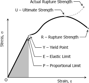
Proportional Limit (Hooke’s Law):
From the origin O to the point called proportional limit, the stress-strain curve is a straight line. This linear relation between elongation and the axial force causing was first noticed by Sir Robert Hooke in 1678 and is called Hooke’s Law that within the proportional limit, the stress is directly proportional to strain or
σ=kε
The constant of proportionality k is called the Modulus of Elasticity E or Young’s Modulus and is equal to the slope of the stress-strain diagram from O to P. Then
σ=Eε
Elastic Limit:
The elastic limit is the limit beyond which the material will no longer go back to its original shape when the load is removed, or it is the maximum stress that may e developed such that there is no permanent or residual deformation when the load is entirely removed.
Elastic and Plastic Ranges:
The region in stress-strain diagram from O to P is called the elastic range. The region from P to R is called the plastic range.
Yield Point:
Yield point is the point at which the material will have an appreciable elongation or yielding without any increase in load.
Ultimate Strength:
The maximum ordinate in the stress-strain diagram is the ultimate strength or tensile strength.
Rapture Strength:
Rapture strength is the strength of the material at rupture. This is also known as the breaking strength.
Modulus of Resilience:
Modulus of resilience is the work done on a unit volume of material as the force is gradually increased from O to P, in N·m/m3. This may be calculated as the area under the stress-strain curve from the origin O to up to the elastic limit E (the shaded area in the figure). The resilience of the material is its ability to absorb energy without creating a permanent distortion.
Modulus of Toughness:
Modulus of toughness is the work done on a unit volume of material as the force is gradually increased from O to R, in N·m/m3. This may be calculated as the area under the entire stress-strain curve (from O to R). The toughness of a material is its ability to absorb energy without causing it to break.
Working Stress, Allowable Stress, and Factor of Safety:
Working stress is defined as the actual stress of a material under a given loading. The maximum safe stress that a material can carry is termed as the allowable stress. The allowable stress should be limited to values not exceeding the proportional limit. However, since proportional limit is difficult to determine accurately, the allowable tress is taken as either the yield point or ultimate strength divided by a factor of safety. The ratio of this strength (ultimate or yield strength) to allowable strength is called the factor of safety.
Introduction to Heat Pipes
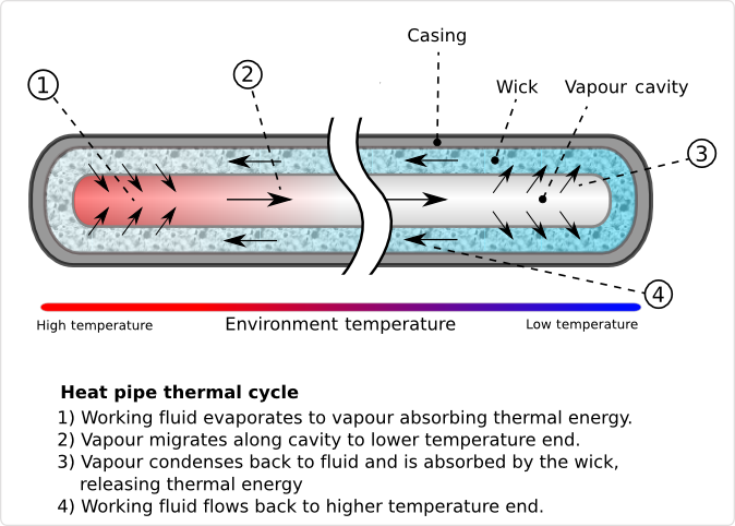
Heat pipes are hollow metal pipes filled with a liquid coolant that moves heat by evaporating and condensing in an endless cycle. A Heat-pipe can be considered a passive heat pump, moving heat as a result of the laws of physics.
As the lower end of the Heat-pipe is exposed to heat, the coolant within it starts to evaporate, absorbing heat. As the coolant turns into vapor, it, and its heat-load, convect within the heat-pipe. The reduced molecular density forces the vaporized coolant upwards, where it is exposed to the cold end of the Heat pipe. The coolant then condenses back into a liquid state, releasing the latent heat. Since the rate of condensation increases with increased delta temperatures between the vapor and Heat pipe surface, the gaseous coolant automatically streams towards the coldest spot within the Heat pipe. As the coolant condenses, and its molecular density increases once more, gravitational forces pull the coolant towards the lower end of the Heat pipe. To aid this coolant cycle, improve its performance, and make it less dependent on the orientation of the Heat pipe towards earth gravitational center, modern Heat-pipes feature inner walls with a fine, capillary structure. The capillary surfaces within the Heat-pipe break the coolants surface tension, distributing it evenly throughout the structure. As soon as coolant evaporates on one end, the coolants surface tension automatically pulls in fresh coolant from the surrounding area. As a result of the self organizing streams of the coolant in both phases, heat is actively convecting through Heat pipes throughout the entire coolant cycle, at a rate unmatched by solid Heat spreaders and Heat sinks.
Heat pipes are a smart investment if you have a device or platform that needs any of the following support:
- Transfer of heat from one location to another. For example, many electronics use this to transfer heat from a chip to a remote heat sink.
- Transform heat from a high heat flux at the evaporator to a lower heat flux at the condenser, making it easier to remove overall heat with conventional methods such as liquid or air cooling. Heat fluxes of up to 1,000 W/cm2 can be transformed with custom vapor chambers.
- Provide an isothermal surface. Examples include operating multiple laser diodes at the same temperature, and providing very isothermal surfaces for temperature calibration.
There are some universal benefits of how a heat pipe works across almost all applications:
- High Effective Thermal Conductivity. Transfer heat over long distances, with minimal temperature drop.
- Passive operation. No moving parts, and require no energy input other than heat to operate.
- Isothermal operation. Very isothermal surfaces, with temperature variations as low as ± 5 mK.
- Long life with no maintenance. No moving parts that could wear out. The vacuum seal prevents liquid losses, and protective coatings can give each device a long-lasting guard against corrosion.
- Lower costs. By lowering the operating temperature, these devices can increase the Mean Time Between Failure (MT-BF) for electronic assemblies. In turn, this lowers the maintenance required, and the replacement costs. In H VAC systems, they can reduce the energy required for heating and air conditioning, with payback times of a few years.
Heat Transfer Limitations of Heat Pipes
Capillary Limit:
The ability of a particular capillary structure to provide the circulation for a given working fluid is limited. This limit is commonly called the capillary limitation or hydrodynamic limitation. The capillary limit is the most commonly encountered limitation in the operation of low-temperature heat pipes. It occurs when the pumping rate is not sufficient to provide enough liquid to the evaporator section. This is due to the fact that the sum of the liquid and vapor pressure drops exceed the maximum capillary pressure that the wick can sustain. The maximum capillary pressure for a given wick structure depends on the physical properties of the wick and working fluid. Any attempt to increase the heat transfer above the capillary limit will cause dry-out in the evaporator section, where a sudden increase in wall temperature along the evaporator section takes place.
Sonic Limit:
The evaporator and condenser sections of a heat pipe represent a vapor flow channel with mass addition and extraction due to the evaporation and condensation, respectively. The vapor velocity increases along the evaporator and reaches a maximum at the end of the evaporator section. The limitation of such a flow system is similar to that of a converging-diverging nozzle with a constant mass flow rate, where the evaporator exit corresponds to the throat of the nozzle. Therefore, one expects that the vapor velocity at that point cannot exceed the local speed of sound. This choked flow condition is called the sonic limitation. The sonic limit usually occurs either during heat pipe startup or during steady state operation when the heat transfer coefficient at the condenser is high. The sonic limit is usually associated with liquid-metal heat pipes due to high vapor velocities and low densities. Unlike the capillary limit, when the sonic limit is exceeded, it does not represent a serious failure. The sonic limitation corresponds to a given evaporator end cap temperature. Increasing the evaporator end cap temperature will increase this limit to a new higher sonic limit. The rate of heat transfer will not increase by decreasing the condenser temperature under the choked condition. Therefore, when the sonic limit is reached, further increases in the heat transfer rate can be realized only when the evaporator temperature increases. Operation of heat pipes with a heat rate close to or at the sonic limit results in a significant axial temperature drop along the heat pipe.
Boiling Limit:
If the radial heat flux in the evaporator section becomes too high, the liquid in the evaporator wick boils and the wall temperature becomes excessively high. The vapor bubbles that form in the wick prevent the liquid from wetting the pipe wall, which causes hot spots. If this boiling is severe, it dries out the wick in the evaporator, which is defined as the boiling limit. However, under a low or moderate radial heat flux, low intensity stable boiling is possible without causing dry-out. It should be noted that the boiling limitation is a radial heat flux limitation as compared to an axial heat flux limitation for the other heat pipe limits. However, since they are related through the evaporator surface area, the maximum radial heat flux limitation also specifies the maximum axial heat transport. The boiling limit is often associated with heat pipes of non-metallic working fluids. For liquid-metal heat pipes, the boiling limit is rarely seen.
Entrainment Limit:
A shear force exists at the liquid-vapor interface since the vapor and liquid move in opposite directions. At high relative velocities, droplets of liquid can be torn from the wick surface and entrained into the vapor flowing toward the condenser section. If the entrainment becomes too great, the evaporator will dry out. The heat transfer rate at which this occurs is called the entrainment limit. Entrainment can be detected by the sounds made by droplets striking the condenser end of the heat pipe. The entrainment limit is often associated with low or moderate temperature heat pipes with small diameters, or high temperature heat pipes when the heat input at the evaporator is high.
Vapor Pressure Limit:
At low operating temperatures, viscous forces may be dominant for the vapor moving flow down the heat pipe. For a long liquid-metal heat pipe, the vapor pressure at the condenser end may reduce to zero. The heat transport of the heat pipe may be limited under this condition. The vapor pressure limit (viscous limit) is encountered when a heat pipe operates at temperatures below its normal operating range, such as during startup from the frozen state. In this case, the vapor pressure is very small, with the condenser end cap pressure nearly zero.
Frozen Startup Limit:
During the startup process from the frozen state, the active length of the heat pipe is less than the total length, and the distance the liquid has to travel in the wick is less than that required for steady state operations. Therefore, the capillary limit will usually not occur during the startup process if the heat input is not very high and is not applied too abruptly. However, for heat pipes with an initially frozen working fluid, if the melting temperature of the working fluid and the heat capacities of the heat pipe container and wick are high, and the latent heat of evaporation and cross-sectional area of the wick are small, a frozen startup limit may occur due to the freezing out of vapor from the evaporation zone to the adiabatic or condensation zone.
Condenser Heat Transfer Limit:
In general, heat pipe condensers and the method of cooling the condenser should be designed such that the maximum heat rate capable of being transported by the heat pipe can be removed. However, in exceptional cases with high temperature heat pipes, appropriate condensers cannot be developed to remove the maximum heat capability of the heat pipe. Due to the presence of noncondensible gases, the effective length of the heat pipe is reduced during continuous operation. Therefore, the condenser is not used to its full capacity. In both cases, the heat transfer limitation can be due to the condenser limit.
Vapor Continuum Limit:
For heat pipes with very low operating temperatures, especially when the dimension of the heat pipe is very small such as micro heat pipes, the vapor flow in the heat pipe may be in the free molecular or rarefied condition. The heat transport capability under this condition is limited, and is called the vapor continuum limit.
Flooding Limit:
The flooding limit is the most common concern for long thermosyphons with large liquid fill ratios, large axial heat fluxes, and small radial heat fluxes. This limit occurs due to the instability of the liquid film generated by a high value of inter-facial shear, which is a result of the large vapor velocities induced by high axial heat fluxes. The vapor shear hold-up prevents the condensate from returning to the evaporator and leads to a flooding condition in the condenser section. This causes a partial dry-out of the evaporator, which results in wall temperature excursions or in limiting the operation of the system.
Heat pipe heat sink:

Graphene under pressure
Small balloons made from one-atom-thick material graphene can withstand enormous pressures, much higher than those at the bottom of the deepest ocean, scientists at the University of Manchester report.
This is due to graphene’s incredible strength – 200 times stronger than steel.
The graphene balloons routinely form when placing graphene on flat substrates and are usually considered a nuisance and therefore ignored. The Manchester researchers, led by Professor Irina Grigorieva, took a closer look at the nano-bubbles and revealed their fascinating properties.
These bubbles could be created intentionally to make tiny pressure machines capable of withstanding enormous pressures. This could be a significant step towards rapidly detecting how molecules react under extreme pressure.
Writing in Nature Communications, the scientists found that the shape and dimensions of the nano-bubbles provide straightforward information about both graphene’s elastic strength and its interaction with the underlying substrate.
The researchers found such balloons can also be created with other two-dimensional crystals such as single layers of molybdenum disulfide (MoS2) or boron nitride.
They were able to directly measure the pressure exerted by graphene on a material trapped inside the balloons, or vice versa.
To do this, the team indented bubbles made by graphene, mono-layer MoS2 and mono-layer boron nitride using a tip of an atomic force microscope and measured the force that was necessary to make a dent of a certain size.
These measurements revealed that graphene enclosing bubbles of a micron size creates pressures as high as 200 mega-pascals, or 2,000 atmospheres. Even higher pressures are expected for smaller bubbles.
Ekaterina Khestanova, a PhD student who carried out the experiments, said: “Such pressures are enough to modify the properties of a material trapped inside the bubbles and, for example, can force crystallization of a liquid well above its normal freezing temperature’.
Sir Andre Geim, a co-author of the paper, added: “Those balloons are ubiquitous. One can now start thinking about creating them intentionally to change enclosed materials or study the properties of atomically thin membranes under high strain and pressure.”
Introduction to machine tool / Single point cutting tool
The tool is wedge shape object of hard material. It is usually made from H.S.S. Beside H.S.S. machine tool is also made from High Carbon Steel, Satellite, Ceramics, Diamond, Abrasive, etc. The main requirement of tool material is hardness. It must be hard enough to resist cutting forces applied on work piece. Hot hardness, wear resistance, Toughness, Thermal conductivity, & specific heat, coefficient of friction, are other requirement of tool material. All these properties should be high.
Classification of cutting tools
A] According to number of cutting edge.
Single point cutting tool
It is simplest from of cutting tool & it have only one cutting edge.
Examples – shear tools, lathe tools, planer tools, boring tolls etc.
Multi point cutting tool
In this two or more single point cutting tools arranged together as a unit. The rate of machining is more & surface finish is also better in this case.
Example- milling cutter, drills, brooches, grinding wheels, abrasive sticks etc.
B] According to motion
Linear motion tools – lathe tools, brooches
Rotary motion tools – milling cutters, grinding wheels
Linear & rotary motion tools – drills, taps, etc.
Single point cutting tool geometry
The single point cutting tool mainly consist of tool shank & cutting part called point. The point of cutting tool is bounded by cutting face, end flank, side/ main flank, & base. The chip slide along the face.
The side / main cutting edge ‘ab’ is formed by intersecting of face & side / main flank
The end cutting edge ‘ac’ is formed by the intersection of end flank & base.
The point ‘a’ which the intersection of end cutting edge & side cutting edge is called nose
Mainly the chip cuts by side cutting edge.
Terminology of single point cutting tool
Shank – It is main body of tool. The shank used to gripped in tool holder.
Flank – The surface or surface below the adjacent of the cutting edge is called flank of the tool.
Face – It is top surface of the tool along which the chips slides.
Base – It is actually a bearing surface of the tool when it is held in tool holder or clamped directly in a tool post.
Heel – It is the intersection of the flank & base of the tool. It is curved portion at the bottom of the tool.
Nose – It is the point where side cutting edge & base cutting edge intersect.
Cutting edge – It is the edge on face of the tool which removes the material from work-piece. The cutting edges are side cutting edge (major cutting edge) & end cutting edge ( minor cutting edge)
Tool angles-Tool angles have great importance. The tool with proper angle, reduce breaking of tool, cut metal more efficiently, generate less heat.
Noise radius –It provide long life & good surface finish sharp point on nose is highly stressed, & leaves grooves in the path of cut.Longer nose radius produce chatter.
Researchers developing new thermal interface materials
In the microelectronics world, the military and private sectors alike need solutions to technological challenges. Dr. Mustafa Akbulut, assistant professor of chemical engineering, and two students lead a project funded by DARPA to create thermal interface materials (TIMs) that have a superior ability to transfer heat and a strong capacity to keep cool.
In evaluating a central processing unit, as an example, there are many pieces that individually need temperature management. “As you get smaller and smaller, there is higher heat dissipation per unit area. Locally, you have higher temperatures…you have a harder time operationally—you need better thermal interface materials. This is especially important for radars, laser systems and also for military electronics,” said Akbulut.
Essentially and most critically, the device needs the ability to avoid overheating. As Akbulut asserts, “unless you cool it, it fails.”
In evaluating an electronic device and a cooling system that need to be placed together as they function, if there is an absence of thermal material in between, the heat created by the electronic device can potentially erode the device. According to Akbulut, non-soft materials are considered less effective as a TIM because they do not adequately cover all interior openings or gaps, even though the naked eye may not detect this space.
Akbulut explains why optimal contact is not achieved through current technology. “If you look at the very fine scale, [these two pieces] are not smooth. If you look at these with an electron microscope, you see they are like mountains. If you bring these surfaces together, they do not have perfect contact.” Thus, the objective of a traditional TIM is not fully met.
Soft materials, including paste, often minimize the gap, said Akbulut. The invention of his new metal-based, soft material leads to high thermal conductive activity and because of its malleable nature, consistent contact is achieved. His research group has recently developed TIMs with thermal conductivities greater than 100 W/m-k and elastic modulus values in the order of 20 GPa, signficantly advancing the current state of art for TIMs. As a comparison, this material is ten times softer than steel and three times more thermally conductive.
Using copper and nanomaterials together, Akbulut believes his new TIM can lead to greater optimization and large-scale implementation in the future.
Fundamentals of Thermal Resistance
The Thermal Resistance Analogy
Thermal resistance is a convenient way of analyzing some heat transfer problems using an electrical analogy in order to make complicated systems easier to visualize and analyze. It is based on an analogy with Ohm’s law which is:
In Ohm’s law for electricity, “V” is the voltage which drives a current of magnitude “I”. The amount of current that flows for a given voltage is proportional to the resistance (Relec). For an electrical conductor, the resistance depends on the material properties (copper tends to have a lower resistance than wood, for example) and the physical configuration (thick short wires have less resistance than long thin wires).
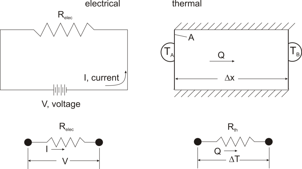
For one-dimensional, steady-state heat transfer problems with no internal heat generation, the heat flow is proportional to a temperature difference according to this equation:
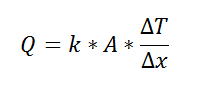
where Q is the heat flow, k is the material property of thermal conductivity, A is the area normal to the flow of heat, Δx is the distance that the heat flows, and ΔT is the temperature difference driving the heat flow.
If we create an analogy by saying that electrical current flows like heat, and saying that voltage drives the electrical current like the temperature difference drives the heat flow, we can write the heat flow equation in a form similar to Ohm’s law: 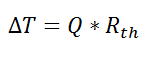 where Rth is the thermal resistance defined as:
 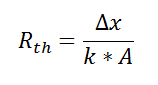 Just as with the electrical resistance, the thermal resistance will be higher for a small cross-sectional area of heat flow (A) or for a long distance (Δx).
Rationale
Now, why bother with all that? The answer is that thermal resistance allows us to solve somewhat complicated problems in relatively simple ways. We’ll talk more about different ways in which it can be used, but first let’s look at a simple case in order to illustrate the benefit.
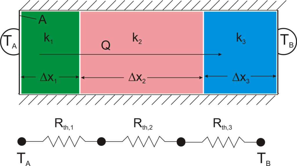
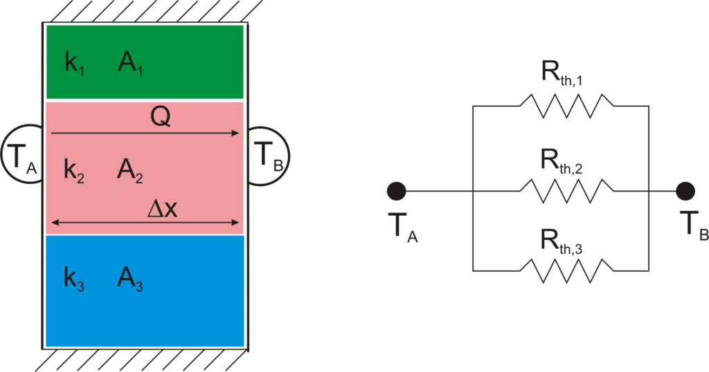
Suppose that we want to calculate the heat flow through a wall composed of three different materials, and we know the surface temperatures at each outside surface, TA, and TB, and the material properties and geometries.
We could write the conduction equation for each material:
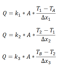
Now, we have three equations, and three unknowns: T1, T2, and Q. For this case it wouldn’t be too much work to algebraically solve for those three unknowns, however, if we use the thermal resistance analogy, we don’t even have to do that much work:
![]()
where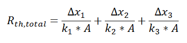
and we can solve for Q in a single step.
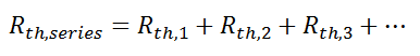
Combining Thermal Resistances
This simple example showed how to combine multiple thermal resistances in series which is the same structure as in the electrical analog:
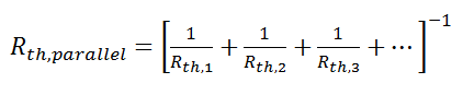
Just like electrical resistances, thermal resistances can also be combined in parallel, or in both series and parallel:

Beyond Conduction
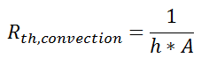
So far, we’ve talked about the thermal resistance associated with conduction through a plane wall. For steady-state, one-dimensional problems, other heat transfer equations can be formulated into a thermal resistance format. For example, examine Newton’s Law of Cooling for convection heat transfer:
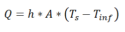
where Q is the heat flow, h is the convective heat transfer coefficient, A is the area over which heat transfer occurs, Ts is the surface temperature on which the convection is taking place, and Tinf is the free-stream temperature of the fluid. As with conduction, there is a temperature difference driving a heat flow. For this case, the thermal resistance would be:
Similarly, for radiative heat transfer from a gray body:
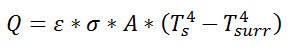
where Q is the heat flow, ε is the emissivity of the surface, σ is the Stefan-Boltzmann constant, Ts is the surface temperature of the emitting surface, and Tsurr is the temperature of the surroundings. By factoring the expression for temperature, the thermal resistance can be written: 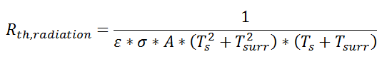
Advantage: Easy Problem Setup
Thermal resistance formulations can make the arrangement of a quite complex problem quite simple to set up. Imagine, for example, that we are trying to calculate the heat flow from a liquid stream of a known temperature through a composite wall to an air stream with convection and radiation occurring on the air side. If the material properties, heat transfer coefficients, and geometry are known, the equation set-up is obvious:
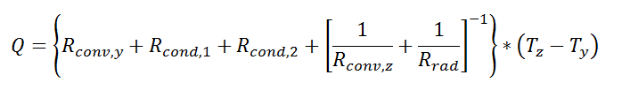
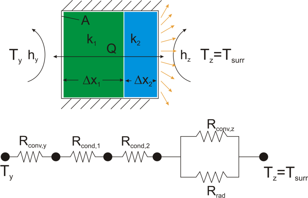
Now, to solve this particular problem might involve an iterative solution since the radiative thermal resistance contains the surface temperature inside of it, but the setup is simple and straightforward.
Advantage: Problem Insight
The thermal resistance formulation has the additional advantage of making it very clear which parts of the model are controlling the heat transfer, and which parts are unimportant, or perhaps even negligible. As a concrete illustration, let’s suppose that in the last example the thermal resistance on the liquid side was 20 K/W, that the first layer in the composite wall was 1 mm thick plastic with a thermal resistance of 40 K/W, that the second layer consisted of 2 mm thick steel with a thermal resistance of 0.5 K/W, and that the thermal resistance for convection to the air was 200 K/W, and the thermal resistance to radiation to the surroundings was 2500 K/W coming from a surface with emissivity of 0.5.
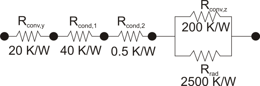
We can understand a lot about the problem by just considering the thermal resistance. For example, since the radiation resistance is in parallel with a much smaller convection resistance, it is going to have a small effect on the overall thermal resistance. Increasing the emissivity of the wall clear to unity would only improve the total thermal resistance by 5%. Or, ignoring radiation completely would cause an error of only 6%. Similarly, the thermal resistance of the steel is in series, and is tiny compared with the other resistances in the system, so no matter what is done to the metal layer it isn’t going to have much effect. Changing from steel to pure copper, for example, would only improve the overall thermal resistance by 0.2%. Finally, it is clear that the controlling thermal resistance is convection on the air side. If it were possible to double the convection coefficient (by, say, increasing the velocity of the air) that step alone would decrease the overall thermal resistance by 36%.
Beyond Plane Wall Conduction
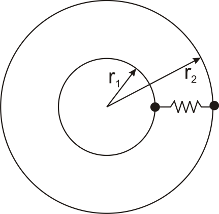
Thermal resistance can also be used for other conduction geometries as long as they can be analyzed as one-dimensional. The thermal resistance to conduction in a cylindrical geometry is:
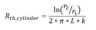
where L is the axial distance along the cylinder, and r1 and r2 are as shown in the figure.
Thermal resistance for a spherical geometry is:
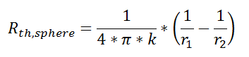
with r1 and r2 as shown in the figure.
Conclusion
Thermal resistance is a powerful and useful tool for analyzing problems that can be approximated as 1-dimensional, steady-state, and that do not have any sources of heat generation.