Category: Basic Thermal Engineering

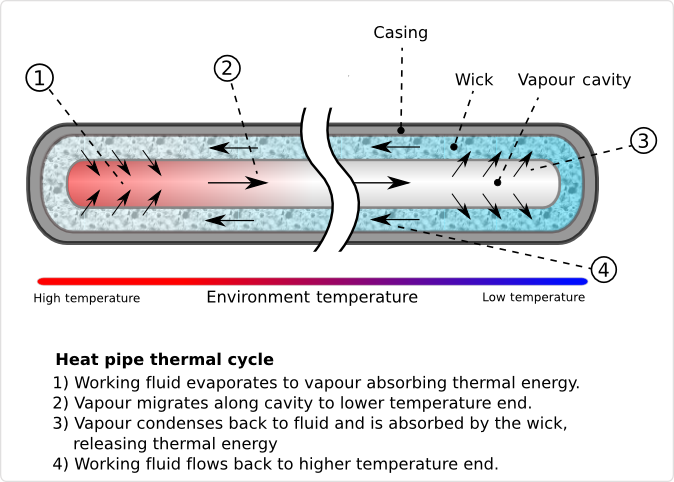
Heat pipes are hollow metal pipes filled with a liquid coolant that moves heat by evaporating and condensing in an endless cycle. A Heat-pipe can be considered a passive heat pump, moving heat as a result of the laws of physics.

As the lower end of the Heat-pipe is exposed to heat, the coolant within it starts to evaporate, absorbing heat. As the coolant turns into vapor, it, and its heat-load, convect within the heat-pipe. The reduced molecular density forces the vaporized coolant upwards, where it is exposed to the cold end of the Heat pipe. The coolant then condenses back into a liquid state, releasing the latent heat. Since the rate of condensation increases with increased delta temperatures between the vapor and Heat pipe surface, the gaseous coolant automatically streams towards the coldest spot within the Heat pipe. As the coolant condenses, and its molecular density increases once more, gravitational forces pull the coolant towards the lower end of the Heat pipe. To aid this coolant cycle, improve its performance, and make it less dependent on the orientation of the Heat pipe towards earth gravitational center, modern Heat-pipes feature inner walls with a fine, capillary structure. The capillary surfaces within the Heat-pipe break the coolants surface tension, distributing it evenly throughout the structure. As soon as coolant evaporates on one end, the coolants surface tension automatically pulls in fresh coolant from the surrounding area. As a result of the self organizing streams of the coolant in both phases, heat is actively convecting through Heat pipes throughout the entire coolant cycle, at a rate unmatched by solid Heat spreaders and Heat sinks.

 

 

Heat pipes are a smart investment if you have a device or platform that needs any of the following support:

1. Transfer of heat from one location to another. For example, many electronics use this to transfer heat from a chip to a remote heat sink.
2. Transform heat from a high heat flux at the evaporator to a lower heat flux at the condenser, making it easier to remove overall heat with conventional methods such as liquid or air cooling. Heat fluxes of up to 1,000 W/cm2 can be transformed with custom vapor chambers.
3. Provide an isothermal surface. Examples include operating multiple laser diodes at the same temperature, and providing very isothermal surfaces for temperature calibration.

There are some universal benefits of how a heat pipe works across almost all applications:

1. High Effective Thermal Conductivity. Transfer heat over long distances, with minimal temperature drop.
2. Passive operation. No moving parts, and require no energy input other than heat to operate.
3. Isothermal operation. Very isothermal surfaces, with temperature variations as low as ± 5 mK.
4. Long life with no maintenance. No moving parts that could wear out. The vacuum seal prevents liquid losses, and protective coatings can give each device a long-lasting guard against corrosion.
5. Lower costs. By lowering the operating temperature, these devices can increase the Mean Time Between Failure (MT-BF) for electronic assemblies. In turn, this lowers the maintenance required, and the replacement costs. In H VAC systems, they can reduce the energy required for heating and air conditioning, with payback times of a few years.

Heat Transfer Limitations of Heat Pipes

Capillary Limit:

The ability of a particular capillary structure to provide the circulation for a given working fluid is limited. This limit is commonly called the capillary limitation or hydrodynamic limitation. The capillary limit is the most commonly encountered limitation in the operation of low-temperature heat pipes. It occurs when the pumping rate is not sufficient to provide enough liquid to the evaporator section. This is due to the fact that the sum of the liquid and vapor pressure drops exceed the maximum capillary pressure that the wick can sustain. The maximum capillary pressure for a given wick structure depends on the physical properties of the wick and working fluid. Any attempt to increase the heat transfer above the capillary limit will cause dry-out in the evaporator section, where a sudden increase in wall temperature along the evaporator section takes place.

Sonic Limit:

The evaporator and condenser sections of a heat pipe represent a vapor flow channel with mass addition and extraction due to the evaporation and condensation, respectively. The vapor velocity increases along the evaporator and reaches a maximum at the end of the evaporator section. The limitation of such a flow system is similar to that of a converging-diverging nozzle with a constant mass flow rate, where the evaporator exit corresponds to the throat of the nozzle. Therefore, one expects that the vapor velocity at that point cannot exceed the local speed of sound. This choked flow condition is called the sonic limitation. The sonic limit usually occurs either during heat pipe startup or during steady state operation when the heat transfer coefficient at the condenser is high. The sonic limit is usually associated with liquid-metal heat pipes due to high vapor velocities and low densities. Unlike the capillary limit, when the sonic limit is exceeded, it does not represent a serious failure. The sonic limitation corresponds to a given evaporator end cap temperature. Increasing the evaporator end cap temperature will increase this limit to a new higher sonic limit. The rate of heat transfer will not increase by decreasing the condenser temperature under the choked condition. Therefore, when the sonic limit is reached, further increases in the heat transfer rate can be realized only when the evaporator temperature increases. Operation of heat pipes with a heat rate close to or at the sonic limit results in a significant axial temperature drop along the heat pipe.

Boiling Limit:

If the radial heat flux in the evaporator section becomes too high, the liquid in the evaporator wick boils and the wall temperature becomes excessively high. The vapor bubbles that form in the wick prevent the liquid from wetting the pipe wall, which causes hot spots. If this boiling is severe, it dries out the wick in the evaporator, which is defined as the boiling limit. However, under a low or moderate radial heat flux, low intensity stable boiling is possible without causing dry-out. It should be noted that the boiling limitation is a radial heat flux limitation as compared to an axial heat flux limitation for the other heat pipe limits. However, since they are related through the evaporator surface area, the maximum radial heat flux limitation also specifies the maximum axial heat transport. The boiling limit is often associated with heat pipes of non-metallic working fluids. For liquid-metal heat pipes, the boiling limit is rarely seen.

Entrainment Limit:

A shear force exists at the liquid-vapor interface since the vapor and liquid move in opposite directions. At high relative velocities, droplets of liquid can be torn from the wick surface and entrained into the vapor flowing toward the condenser section. If the entrainment becomes too great, the evaporator will dry out. The heat transfer rate at which this occurs is called the entrainment limit. Entrainment can be detected by the sounds made by droplets striking the condenser end of the heat pipe. The entrainment limit is often associated with low or moderate temperature heat pipes with small diameters, or high temperature heat pipes when the heat input at the evaporator is high.

Vapor Pressure Limit:

At low operating temperatures, viscous forces may be dominant for the vapor moving flow down the heat pipe. For a long liquid-metal heat pipe, the vapor pressure at the condenser end may reduce to zero. The heat transport of the heat pipe may be limited under this condition. The vapor pressure limit (viscous limit) is encountered when a heat pipe operates at temperatures below its normal operating range, such as during startup from the frozen state. In this case, the vapor pressure is very small, with the condenser end cap pressure nearly zero.

Frozen Startup Limit:

During the startup process from the frozen state, the active length of the heat pipe is less than the total length, and the distance the liquid has to travel in the wick is less than that required for steady state operations. Therefore, the capillary limit will usually not occur during the startup process if the heat input is not very high and is not applied too abruptly. However, for heat pipes with an initially frozen working fluid, if the melting temperature of the working fluid and the heat capacities of the heat pipe container and wick are high, and the latent heat of evaporation and cross-sectional area of the wick are small, a frozen startup limit may occur due to the freezing out of vapor from the evaporation zone to the adiabatic or condensation zone.

Condenser Heat Transfer Limit:

In general, heat pipe condensers and the method of cooling the condenser should be designed such that the maximum heat rate capable of being transported by the heat pipe can be removed. However, in exceptional cases with high temperature heat pipes, appropriate condensers cannot be developed to remove the maximum heat capability of the heat pipe. Due to the presence of noncondensible gases, the effective length of the heat pipe is reduced during continuous operation. Therefore, the condenser is not used to its full capacity. In both cases, the heat transfer limitation can be due to the condenser limit.

Vapor Continuum Limit:

For heat pipes with very low operating temperatures, especially when the dimension of the heat pipe is very small such as micro heat pipes, the vapor flow in the heat pipe may be in the free molecular or rarefied condition. The heat transport capability under this condition is limited, and is called the vapor continuum limit.

Flooding Limit:

The flooding limit is the most common concern for long thermosyphons with large liquid fill ratios, large axial heat fluxes, and small radial heat fluxes. This limit occurs due to the instability of the liquid film generated by a high value of inter-facial shear, which is a result of the large vapor velocities induced by high axial heat fluxes. The vapor shear hold-up prevents the condensate from returning to the evaporator and leads to a flooding condition in the condenser section. This causes a partial dry-out of the evaporator, which results in wall temperature excursions or in limiting the operation of the system.

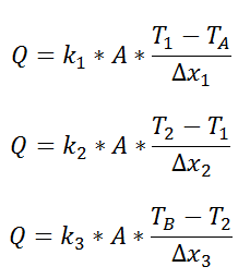
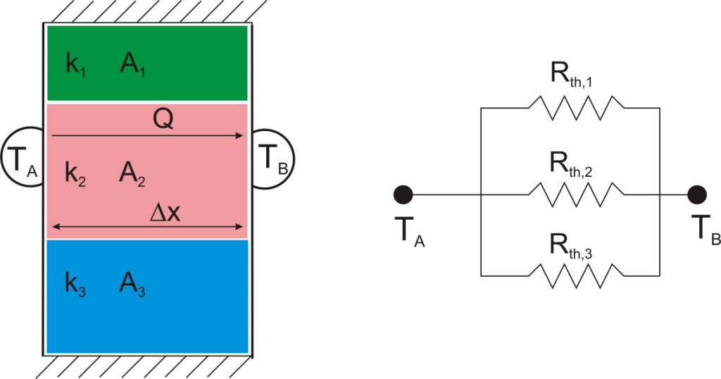
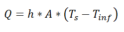
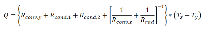
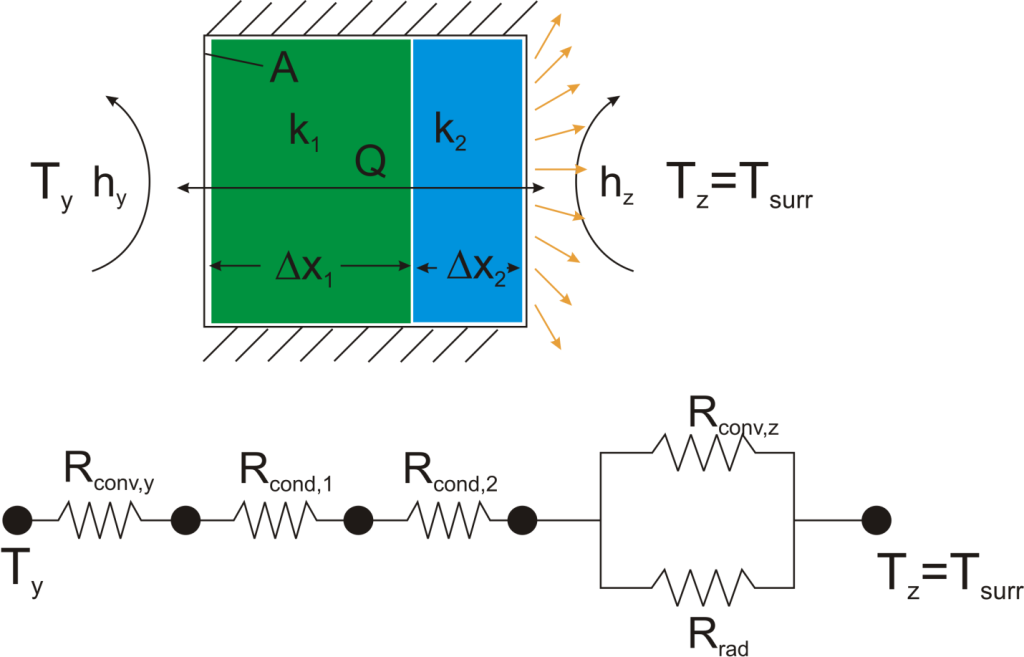
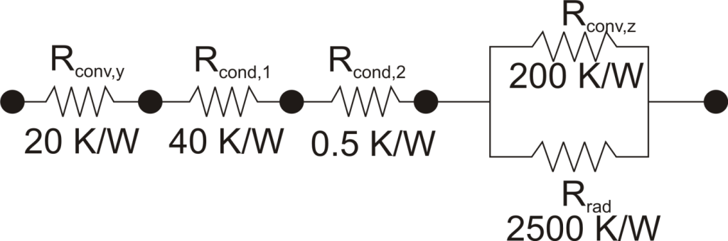
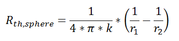
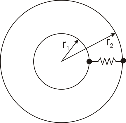
Heat pipe heat sink:

 

 

The Thermal Resistance Analogy

Thermal resistance is a convenient way of analyzing some heat transfer problems using an electrical analogy in order to make complicated systems easier to visualize and analyze. It is based on an analogy with Ohm’s law which is:

In Ohm’s law for electricity, “V” is the voltage which drives a current of magnitude “I”. The amount of current that flows for a given voltage is proportional to the resistance (R_elec). For an electrical conductor, the resistance depends on the material properties (copper tends to have a lower resistance than wood, for example) and the physical configuration (thick short wires have less resistance than long thin wires).

 

For one-dimensional, steady-state heat transfer problems with no internal heat generation, the heat flow is proportional to a temperature difference according to this equation:

where Q is the heat flow, k is the material property of thermal conductivity, A is the area normal to the flow of heat, Δx is the distance that the heat flows, and ΔT is the temperature difference driving the heat flow.

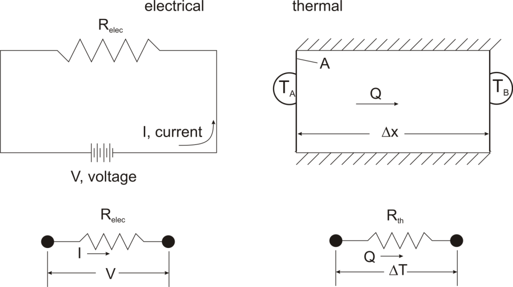
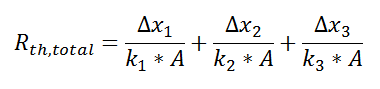
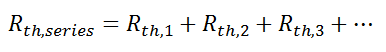
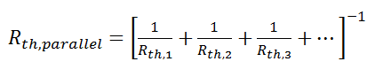
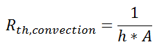
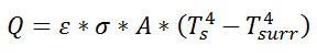
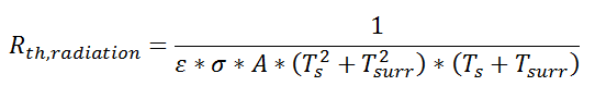
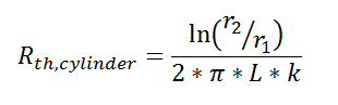
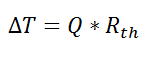
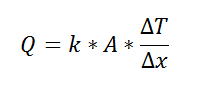
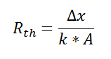
If we create an analogy by saying that electrical current flows like heat, and saying that voltage drives the electrical current like the temperature difference drives the heat flow, we can write the heat flow equation in a form similar to Ohm’s law: where R_th is the thermal resistance defined as: Just as with the electrical resistance, the thermal resistance will be higher for a small cross-sectional area of heat flow (A) or for a long distance (Δx).

Rationale

Now, why bother with all that? The answer is that thermal resistance allows us to solve somewhat complicated problems in relatively simple ways. We’ll talk more about different ways in which it can be used, but first let’s look at a simple case in order to illustrate the benefit.

Suppose that we want to calculate the heat flow through a wall composed of three different materials, and we know the surface temperatures at each outside surface, T_A, and T_B, and the material properties and geometries.

 

We could write the conduction equation for each material:

Now, we have three equations, and three unknowns: T₁, T₂, and Q. For this case it wouldn’t be too much work to algebraically solve for those three unknowns, however, if we use the thermal resistance analogy, we don’t even have to do that much work:

where

and we can solve for Q in a single step.

Combining Thermal Resistances

This simple example showed how to combine multiple thermal resistances in series which is the same structure as in the electrical analog:

Just like electrical resistances, thermal resistances can also be combined in parallel, or in both series and parallel:

Beyond Conduction

So far, we’ve talked about the thermal resistance associated with conduction through a plane wall. For steady-state, one-dimensional problems, other heat transfer equations can be formulated into a thermal resistance format. For example, examine Newton’s Law of Cooling for convection heat transfer:

where Q is the heat flow, h is the convective heat transfer coefficient, A is the area over which heat transfer occurs, T_s is the surface temperature on which the convection is taking place, and T_inf is the free-stream temperature of the fluid. As with conduction, there is a temperature difference driving a heat flow. For this case, the thermal resistance would be:

Similarly, for radiative heat transfer from a gray body:

where Q is the heat flow, ε is the emissivity of the surface, σ is the Stefan-Boltzmann constant, T_s is the surface temperature of the emitting surface, and T_surr is the temperature of the surroundings. By factoring the expression for temperature, the thermal resistance can be written: 

Advantage: Easy Problem Setup

Thermal resistance formulations can make the arrangement of a quite complex problem quite simple to set up. Imagine, for example, that we are trying to calculate the heat flow from a liquid stream of a known temperature through a composite wall to an air stream with convection and radiation occurring on the air side. If the material properties, heat transfer coefficients, and geometry are known, the equation set-up is obvious:

 

 

Now, to solve this particular problem might involve an iterative solution since the radiative thermal resistance contains the surface temperature inside of it, but the setup is simple and straightforward.

Advantage: Problem Insight
The thermal resistance formulation has the additional advantage of making it very clear which parts of the model are controlling the heat transfer, and which parts are unimportant, or perhaps even negligible. As a concrete illustration, let’s suppose that in the last example the thermal resistance on the liquid side was 20 K/W, that the first layer in the composite wall was 1 mm thick plastic with a thermal resistance of 40 K/W, that the second layer consisted of 2 mm thick steel with a thermal resistance of 0.5 K/W, and that the thermal resistance for convection to the air was 200 K/W, and the thermal resistance to radiation to the surroundings was 2500 K/W coming from a surface with emissivity of 0.5.

 

We can understand a lot about the problem by just considering the thermal resistance. For example, since the radiation resistance is in parallel with a much smaller convection resistance, it is going to have a small effect on the overall thermal resistance. Increasing the emissivity of the wall clear to unity would only improve the total thermal resistance by 5%. Or, ignoring radiation completely would cause an error of only 6%. Similarly, the thermal resistance of the steel is in series, and is tiny compared with the other resistances in the system, so no matter what is done to the metal layer it isn’t going to have much effect. Changing from steel to pure copper, for example, would only improve the overall thermal resistance by 0.2%. Finally, it is clear that the controlling thermal resistance is convection on the air side. If it were possible to double the convection coefficient (by, say, increasing the velocity of the air) that step alone would decrease the overall thermal resistance by 36%.

Beyond Plane Wall Conduction

Thermal resistance can also be used for other conduction geometries as long as they can be analyzed as one-dimensional. The thermal resistance to conduction in a cylindrical geometry is:

where L is the axial distance along the cylinder, and r₁ and r₂ are as shown in the figure.

Thermal resistance for a spherical geometry is:

with r₁ and r₂ as shown in the figure.

Conclusion

Thermal resistance is a powerful and useful tool for analyzing problems that can be approximated as 1-dimensional, steady-state, and that do not have any sources of heat generation.

In heat transfer at a boundary (surface) within a fluid, the Nusselt number (Nu) is the ratio of convective to conductive heat transfer across (normal to) the boundary. In this context, convection includes both advection and diffusion. Named after Wilhelm Nusselt, it is a dimensionless number. The conductive component is measured under the same conditions as the heat convection but with a (hypothetically) stagnant (or motionless) fluid. A similar non-dimensional parameter is Biot Number, with the difference that the thermal conductivity is of the solid body and not the fluid.

A Nusselt number close to one, namely convection and conduction of similar magnitude, is characteristic of “slug flow” or laminar flow. A larger Nusselt number corresponds to more active convection, with turbulent flow typically in the 100–1000 range.

The convection and conduction heat flows are parallel to each other and to the surface normal of the boundary surface, and are all perpendicular to the mean fluid flow in the simple case.

where h is the convective heat transfer coefficient of the flow, L is the characteristic length, k is the thermal conductivity of the fluid.

Selection of the characteristic length should be in the direction of growth (or thickness) of the boundary layer; some examples of characteristic length are: the outer diameter of a cylinder in (external) cross flow (perpendicular to the cylinder axis), the length of a vertical plate undergoing natural convection, or the diameter of a sphere. For complex shapes, the length may be defined as the volume of the fluid body divided by the surface area.
The thermal conductivity of the fluid is typically (but not always) evaluated at the film temperature, which for engineering purposes may be calculated as the mean-average of the bulk fluid temperature and wall surface temperature.
In contrast to the definition given above, known as average Nusselt number, local Nusselt number is defined by taking the length to be the distance from the surface boundary to the local point of interest.

The mean, or average, number is obtained by integrating the expression over the range of interest, such as:[2]

The mass transfer analog of the Nusselt number is the Sherwood number.

The Prandtl number (Pr) or Prandtl group is a dimensionless number, defined as the ratio of momentum diffusivity to thermal diffusivity. That is, the Prandtl number is given as:

where:

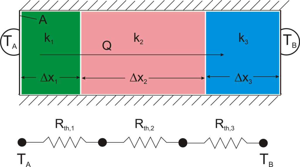
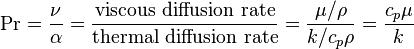
•  : momentum diffusivity (kinematic viscosity), , (SI units: m²/s)
•  : thermal diffusivity, , (SI units: m²/s)
•  : dynamic viscosity, (SI units: Pa s = N s/m²)
•  : thermal conductivity, (SI units: W/m-K)
•  : specific heat, (SI units: J/kg-K)
•  : density, (SI units: kg/m³)

 

Small values of the Prandtl number, Pr << 1, means the thermal diffusivity dominates. Whereas with large values, Pr >> 1, the momentum diffusivity dominates the behavior. For example, for liquid mercury the heat conduction is more significant compared to convection, so thermal diffusivity is dominant. However, for engine oil, convection is very effective in transferring energy from an area in comparison to pure conduction, so momentum diffusivity is dominant.

In heat transfer problems, the Prandtl number controls the relative thickness of the momentum and thermal boundary layers. When Pr is small, it means that the heat diffuses quickly compared to the velocity (momentum). This means that for liquid metals the thickness of the thermal boundary layer is much bigger than the velocity boundary layer.

 

As an object moves through the atmosphere, the gas molecules of the atmosphere near the object are disturbed and move around the object. Aerodynamic forces are generated between the gas and the object. The magnitude of these forces depend on the shape of the object, the speed of the object, the mass of the gas going by the object and on two other important properties of the gas; the viscosity, or stickiness, of the gas and the compressibility, or springiness, of the gas. To properly model these effects, aerodynamicists use similarity parameters which are ratios of these effects to other forces present in the problem. If two experiments have the same values for the similarity parameters, then the relative importance of the forces are being correctly modelled.

Aerodynamic forces depend in a complex way on the viscosity of the gas. As an object moves through a gas, the gas molecules stick to the surface. This creates a layer of air near the surface, called a boundary layer, which, in effect, changes the shape of the object. The flow of gas reacts to the edge of the boundary layer as if it was the physical surface of the object. To make things more confusing, the boundary layer may separate from the body and create an effective shape much different from the physical shape. And to make it even more confusing, the flow conditions in and near the boundary layer are often unsteady (changing in time). The boundary layer is very important in determining the drag of an object. To determine and predict these conditions, aerodynamicists rely on wind tunnel testing and very sophisticated computer analysis.

The important similarity parameter for viscosity is the Reynolds number. The Reynolds number expresses the ratio of inertial (resistant to change or motion) forces to viscous (heavy and gluey) forces. From a detailed analysis of the momentum conservation equation, the inertial forces are characterized by the product of the density rho times the velocity V times the gradient of the velocity dV/dx. The viscous forces are characterized by the dynamic viscosity coefficient mu times the second gradient of the velocity d^2V/dx^2. The Reynolds number Re then becomes:

Re = (rho * V * dV/dx) / (mu * d^2V/dx^2)

The gradient of the velocity is proportional to the velocity divided by a length scale L. Similarly, the second derivative of the velocity is proportional to the velocity divided by the square of the length scale. Then:

Re = (rho * V * V/L) / (mu * V / L^2)

Re = (rho * V * L) / mu

The Reynolds number is a dimensionless number.

The Reynolds number can be further simplified if we use the kinematic viscosity nu that is equal to the dynamic viscosity divided by the density:

nu = mu / rho

Re = V * L / nu

Reynolds Number is used to determine whether a flow will be laminar or turbulent. If Re is high (>2100), inertial forces dominate viscous forces and the flow is turbulent; if Re is low (<1100), viscous forces dominate and the flow is laminar.